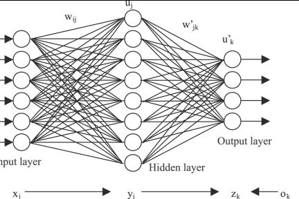
BACKGROUND

A McCulloch Pitts Neuron is a mathematical model of a simulated biological neuron.  It essentially takes in a weighted sum of inputs and calculates an output.

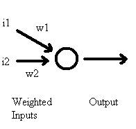
            Figure 1:  A simple model of a biological neuron.  i represents the input (e.g. an

            EPSP),  w represents the synaptic strengths, and output represents some function

            of the neuron’s action potentials.

A Perceptron extends the McCulloch Pitts Neuron with rules for updating the weights based on whether the output of the neuron is favorable or unfavorable.  This is supervised learning.  The output is compared vs. some known target value and errors are corrected. 

A Multi-Layer Perceptron (MLP) links multiple Perceptrons into a network.  More Perceptron units allows for more flexible behavior and pattern storage. 

MECHANISMS

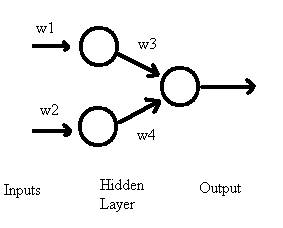
            Figure 2: A simple MultiLayer Perceptron.  The weights are automatically          adjusted based on whether the ultimate output matches some desired target value.         This is supervised learning.

Each neuron’s activity can be calculated independently. 

To calculate each node’s activity (i.e. sum of incoming EPSPs), the weighted sum of inputs are:

                                                                     (1)

            where   means the weighted sum of all inputs i to node j,  is the input    from node i, and   is the weight from node i to node j.

To calculate each node’s output (i.e. whether or not it issues an Action Potential), the node’s processing uses:

                                             (2)

            Which means the output is some function of the activity.  A common function is

            the logistic function:

                                                                        (3)

Which is a sigmoid curve often used in psychology, economics, chemistry, etc.  Its output ranges from [0,1], which is suitable for modeling a probabilistic all-or-none response of an action potential based on EPSPs.  Figure 3 shows a simple example of calculating one node’s output (which loosely resembles the chance it may fire an action potential given its inputs).  The inputs, x, may represent an external stimulus or another node’s output.

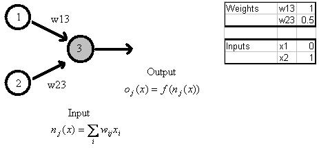
            Figure 3: Demonstration of the output calculations of node j=3 based on weighted

            inputs from nodes 1 and 2.The input, n = (x1*w13)+(x2*w23)=(1*0)+(1*0.5)=0.5

            Logistic function, f(0.5) = 0.63 via equation (3).  This process repeats for each

            neuron, with this output becoming another node’s input where applicable.

Each neuron’s weight update depends on whether it is a hidden or an output node. 

Since an output node’s output can be directly measured against some target value, the error is:

                                          (4)

            Where  is the error for output node j,  is the expected target value,

             is the actual output value, and  is the derivative of the logistic

            function on that node’s input.  f’(x) is defined as:

                                                           (5)

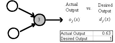
            Figure 4: Demonstration of error term for output node j =3.  From Figure 3, the

            total input n to node 3 is 0.5 and the actual output o from node 3 is 0.63.  If the

            desired output d is 1, the error term is (1-0.63)f’(0.5) = (0.37) [(0.63)(1-0.63)] =         (0.37)(0.63)(0.37) = 0.09.

Since the hidden node’s output only feeds to another node, its output cannot be compared vs. some expected target.  Instead, it uses the errors from all connected downstream nodes:

                                              (6)

            Where is the error for hidden node i,   is the weighted sum of

            errors for all nodes j downstream from this node i.  

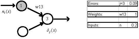
            Figure 5: Demonstration of error term for a hidden node i =1.  From Figure 4, the

            error term for downstream node j=3 was 0.09.  Weight w13 is 1.  If the total    weighted input n to node 1 is 0.2, the error term is (0.09)(1)f’(0.2) =

            (0.09)(0.55)(1-0.55) = (0.09)(0.55)(0.45) = 0.02.

Each weight update depends on its two connected nodes.

For each connection, the weight update is a function of the upstream node’s output and the downstream node’s error. 

                                                                (7)

            where  is some constant learning rate,  is the error from the downstream           node j, and is the output from upstream node i.

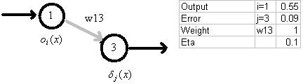
            Figure 6: Demonstration of the weight update for connection from node i to node           j based on upstream node i output and downstream node j error.  From Figure 4,

            the error for node 3 is 0.09.  If weight w13 = 1 and the output from node 1 is 0.55,

            then the weight change = (0.1)(0.09)(0.55) = 0.005.

Summary and Concluding Remarks

To calculate the output, the network processes in feedforward mode:

1. For each node in a given layer, calculate the weighted sum of inputs to that node
2. Use that weighted sum with the logistic function to generate that node’s output

To calculate the weight updates, the network progresses in backwards mode:

3. Calculate the error terms for all output layer nodes
4. Use those error terms to backpropagate and calculate error terms for hidden layer nodes
5. After error terms for each node are calculated, calculate weight updates for each connection between nodes.

The backwards propagating error terms is why this MultiLayer Perceptron model is also known as Backpropagation.